Merge Cubes

This example shows how to merge two synthetic DataCubes, using the dc.merge_cubes() method.

Example

Below is a script that:

• Generates a synthetic data useing generate_pattern_stack().

• Builds two DataCube instances (dc_a and dc_b) with different spatial resolutions and wavelength ranges.

• Displays a side-by-side comparison of a single wavelength slice before resizing.

• Resizes dc_b to match the spatial dimensions of dc_a and displays the aligned slices.

• Merges dc_b into dc_a, producing a combined cube with both wavelength sets.

• Uses the plotter() to visualize the merged cube interactively.

import numpy as np
from wizard import DataCube, plotter
from wizard._utils.example import generate_pattern_stack
from matplotlib.pyplot import subplots, show

# Generate datasets
data_a = generate_pattern_stack(20, 600, 400)
data_b = data_a[:, ::2, ::2]

# Create DataCubes
wls_a = np.linspace(0, 20, 20, dtype=int)
wls_b = np.linspace(60, 100, 20, dtype=int)
dc_a = DataCube(data_a, wavelengths=wls_a, name="dc_a")
dc_b = DataCube(data_b, wavelengths=wls_b, name="dc_b")

# Display cube info
print(dc_a, dc_b, sep='\n')

# Helper for side-by-side comparison
def compare_cubes(c1, c2, idx=1):
    fig, axes = subplots(1, 2, figsize=(10, 5))
    for ax, dc in zip(axes, (c1, c2)):
        ax.imshow(dc[idx])
        ax.set_title(dc.name)
    fig.tight_layout()
    show()

# Initial comparison
compare_cubes(dc_a, dc_b)

# Resize and compare again
dc_b.resize(x_new=dc_a.shape[1], y_new=dc_a.shape[2])
print(dc_b)
compare_cubes(dc_a, dc_b)

# Merge and inspect
dc_a.merge_cubes(dc_b)
print(dc_a)
plotter(dc_a)

Figure Outputs

Figure 1: Initial Comparison

The first figure presents dc_a and dc_b at the same wavelength index. You can see that dc_b (right) has half the resolution of dc_a (left), causing a blockier appearance.

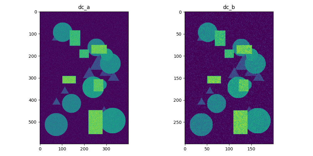
Display cube infos:

Name: dc_a                                          Name: dc_b
Shape: (20, 600, 400)                               Shape: (20, 300, 200)
Wavelengths:                                        Wavelengths:
        Len: 20                                             Len: 20
        From: 0                                             From: 60
        To: 20                                              To: 100

Figure 2: After Resizing

The second figure shows both cubes after calling dc_b.resize(…). Now dc_b matches dc_a in spatial dimensions, and their patterns align perfectly.

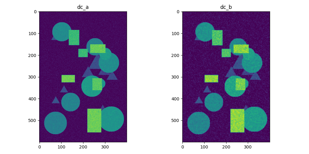
dc_b print output after resize:

Name: dc_b
Shape: (20, 600, 400)
Wavelengths:
       Len: 20
       From: 60
       To: 100

Figure 3: Merged Cube Visualization

After merging, dc_a contains two spectral ranges: the original wavelengths and those from dc_b.

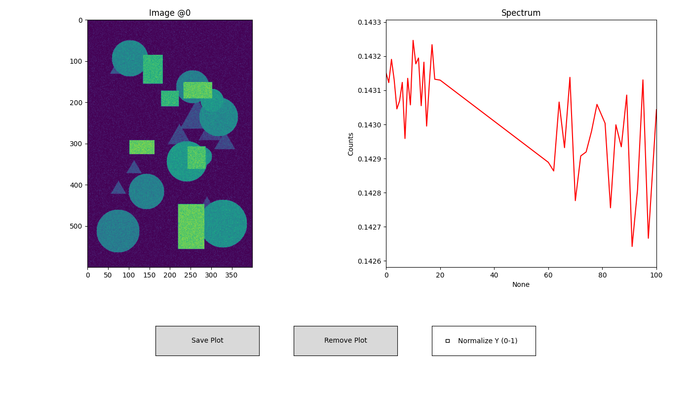
dc_a print output after merge:

Name: dc_a
Shape: (40, 600, 400)
Wavelengths:
       Len: 40
       From: 0
       To: 100