HeiPorSPECTRAL

This example demonstrates the use of the hsi-wizard package to process and visualize biomedical hyperspectral data from the HeiPorSPECTRAL dataset.

The focus is on a spleen tissue scan (sample ID: P086#2021_04_15_09_22_02), part of a collection of annotated hyperspectral scans of human organs. hsi-wizard manages the complete pipeline: reading the raw .dat hyperspectral cube, handling metadata like wavelength calibration, and applying clustering to segment different tissue types based on spectral signatures.

Note

This example uses data from the HeiPorSPECTRAL dataset, published by Studier-Fischer et al. (2023)

Example

The following script demonstrates how to load and analyze a spleen sample from the HeiPorSPECTRAL dataset using hsi-wizard.

"""
This snippet demonstrates the use of the hsi-wizard package for processing and visualizing
hyperspectral data, using a real sample from the HeiPorSPECTRAL dataset [Studier‑Fischer et al., 2023](https://doi.org/10.1038/s41597-023-02315-8).
The focus is on the spleen example (P086#2021_04_15_09_22_02).

The Dataset is availbe on there [Webseite](https://heiporspectral.org)
"""

from matplotlib import pyplot as plt
from matplotlib.colors import ListedColormap
import numpy as np
import wizard
from wizard._processing.cluster import pca, spatial_agglomerative_clustering, smooth_cluster

# Paths
data_path = '2021_04_15_09_22_02_SpecCube.dat'
rgb_path = '2021_04_15_09_22_02_RGB-Image.png'
mask_path = 'HeiPorSPECTRAL_example/data/subjects/P086/2021_04_15_09_22_02/annotations/2021_04_15_09_22_02#polygon#annotator3#spleen#binary.png'

# Load and crop RGB image
rgb_img = plt.imread(rgb_path)[30:-5, 5:-5]
mask = plt.imread(mask_path)

# Create transparent blue colormap
n = 256
alpha_blues = np.zeros((n, 4))
alpha_blues[:, 2] = 1  # Blue channel
alpha_blues[:, 3] = np.linspace(0, 1, n)  # Transparency
t_to_b = ListedColormap(alpha_blues)

# Custom reader
def read_spectral_cube(path) -> wizard.DataCube:
    """
    Read a spectral cube from a binary file and return it as a DataCube object.

    Parameters
    ----------
    path : str
        Path to the binary file containing the spectral cube.

    Returns
    -------
    DataCube
        A wizard.DataCube object

    Credits
    -------
    Inspired by code from: https://github.com/IMSY-DKFZ/htc
    """
    shape = np.fromfile(path, dtype=">i", count=3)
    cube = np.fromfile(path, dtype=">f", offset=12).reshape(*shape)
    cube = np.swapaxes(np.flip(cube, axis=1), 0, 1).astype(np.float32)
    wavelengths = np.linspace(500, 1000, cube.shape[2], dtype='int')
    return wizard.DataCube(cube.transpose(2, 0, 1), wavelengths=wavelengths, notation='nm', name='HeiProSpectral')

# Read data
dc = wizard.DataCube()
dc.set_custom_reader(read_spectral_cube)
dc.custom_read(data_path)

# Inspect Data
wizard.plotter(dc)

# Clustering
dc_pca = pca(dc, n_components=10)
agglo = spatial_agglomerative_clustering(dc_pca, n_clusters=5)
agglo = smooth_cluster(agglo, n_iter=10, sigma=0.5)

# Highlight a specific cluster (e.g., label 2)
highlight = (agglo == 2).astype(float)

# Plot results
fig, axes = plt.subplots(2, 2, figsize=(14, 10))  # 2x2 layout

# Flatten axes array for easier indexing
axes = axes.flatten()

# Update font size for titles
title_fontsize = 14

# Top-left: Original RGB Image
axes[0].imshow(rgb_img)
axes[0].axis('off')
axes[0].set_title('Original RGB Image', fontsize=title_fontsize)

# Bottom-left: RGB with Manual Annotation
axes[1].imshow(rgb_img)
axes[1].imshow(mask, cmap=t_to_b, alpha=0.6)
axes[1].axis('off')
axes[1].set_title('RGB with Manual Annotation', fontsize=title_fontsize)

# Top-right: RGB with Cluster Overlay
axes[3].imshow(rgb_img)
axes[3].imshow(highlight, cmap=t_to_b, alpha=0.6)
axes[3].axis('off')
axes[3].set_title('RGB with Cluster Overlay', fontsize=title_fontsize)

# Bottom-right: Cluster Map
axes[2].imshow(agglo, cmap='cool')
axes[2].axis('off')
axes[2].set_title('Spatial Agglomerative Clustering\non PCA-Reduced Spectral Data (k=5)', fontsize=title_fontsize)

plt.tight_layout()
plt.show()

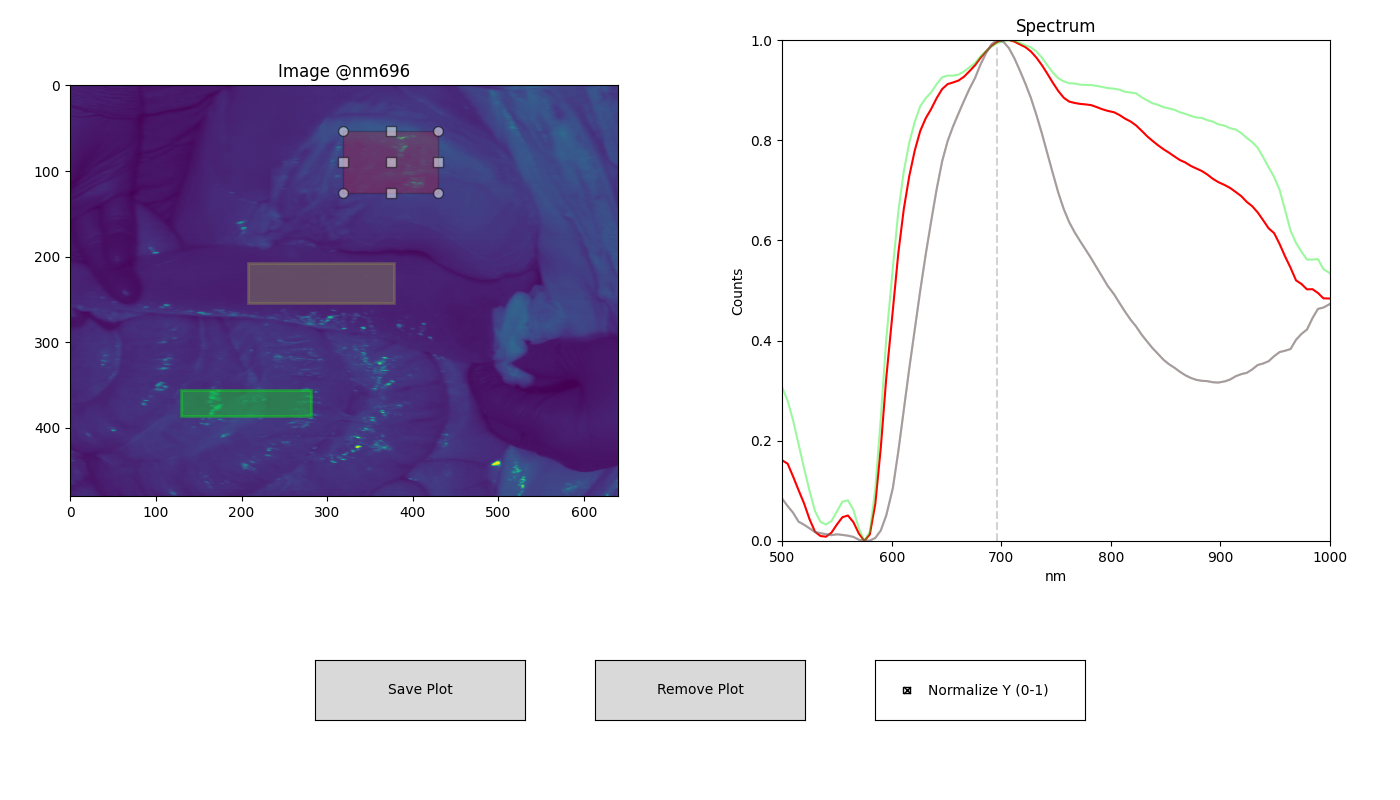
ROI-based spectral analysis using the interactive plotting interface of hsi-wizard. The left panel displays selected tissue regions at 696 nm, while the right panel shows the corresponding normalized spectral profiles.

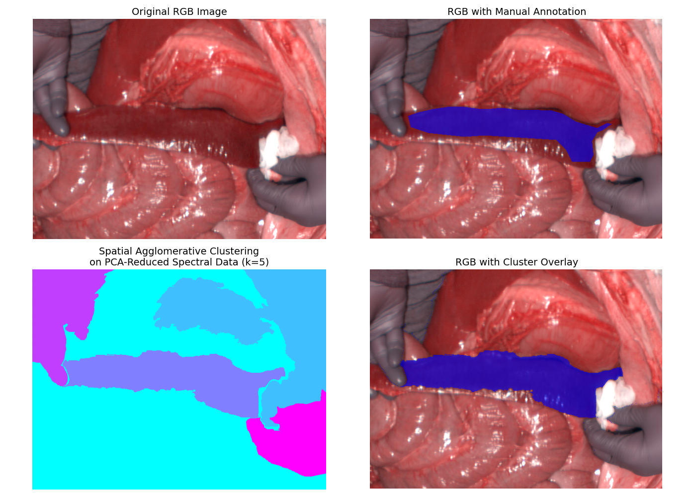
Comparison of manual annotation (top-right) from Studier-Fischer et al. (2023) with automated segmentation (bottom-left) using spatial agglomerative clustering (k = 5). The RGB image (top-left) and the cluster map (bottom-right) offer context and visual feedback for the clustering result.